
Industrial computing codes
General Overview
Course Description
Use of finite element simulation software for mechanics (mainly on Abaqus, a section is devoted to Cast3m). The course will mainly use the graphical interfaces of the different software packages, while also introducing scripting languages for model setup and post-processing, such as Python, Gibiane, etc.
1. Introduction
- Standard modules for defining an elastic analysis (selection of geometry, model, material, and spatial/temporal discretization).
- Assembly creation.
- Domain partitioning.
- Post-processing: field visualization and curve plotting.
2. Advanced Use
- Beams: Slender solids subjected to tension, bending, and torsion using the Bernoulli and Timoshenko beam models. Trusses.
- Plates: Thin solids using the Kirchhoff-Love and Reissner-Mindlin plate models.
- Plasticity: Perfect plasticity. Prandtl-Reuss model.
- Contact: With or without friction. Penalty method or Lagrange multiplier method. Concept of compatible meshing.
- Dynamics: Implicit and explicit methods.
- Vibrations: Natural frequencies and mode shapes.
- Thermal and Thermomechanical Analysis: Heat conduction and thermal expansion.
Prerequisites
Fundamentals of the finite element method.
Learning Objectives
Upon completion of this course, students will be able to:
- Master geometry creation tools: sketching, constraints, dimensions, symmetry, extrusion, revolution, etc.
- Understand the properties of the different finite elements (compatibility, degrees of freedom, integration methods, shape functions, convergence).
- Select appropriate 3D, plate, or beam elements in order to avoid common issues (locking, zero-energy modes).
- Refine meshes to optimize computation time and convergence.
- Simulate nonlinear problems involving contact, plasticity, fracture, etc., under quasi-static or dynamic conditions.
- Use software documentation effectively.
- Perform model setup and post-processing using either the graphical interface or a scripting language.
Session Details
Introduction (5 sessions)
Session 1: General Introduction to Abaqus
Session 2: Part and Property Modules Part Module:
- Sketch creation tool.
- Under-constrained and over-constrained sketches.
- Creation of simple geometries: rectangles and circles.
- Creating cut features to remove material.
- Creation of construction lines.
- Adding dimensions.
- Polyline tool.
- Automatic addition of constraints (right angles).
- RPY file.
- Sketch module.
Property Module:
- Material behavior creation and manager tool.
- Section creation and manager tool.
- Section assignment tool.
Mechanics / Finite Elements:
- Stress-strain law, yield strength, isotropic/kinematic hardening, perfect plasticity.
- Concept of mesh refinement in regions with high gradients.
- Strength of materials and the need to define a section.
Property Module:
- Material orientation assignment tool.
- Geometry partitioning.
- Creation of multiple materials, each assigned to a different part of the geometry.
Application exercise: heat diffusion in a rectangular block.
Beams (4 sessions)
In this part of the course, consisting of four practical sessions, students learn the different methods available in Abaqus for applying beam theory. The theory of beams in tension, bending, and torsion, covered in the Beams and Plates course of the Master 1 SGM program, is assumed to be already familiar to the students. Although beam theory is an approximation, it is widely used in industrial finite element simulations because it drastically reduces mesh density when modeling slender structures, such as steel reinforcement bars embedded in reinforced concrete.
Several types of finite elements based on beam theory are available in Abaqus, including Truss, Beam, and Spring elements, all of which will be used in this course. Students will learn under which circumstances each type of element should be used. Four 3-hour practical sessions are devoted to the study of beams. Sessions 1 and 2 focus on beams under tension and compression, while Sessions 3 and 4 cover bending and torsion in greater detail.
Lab 1: Beams in Tension In the first lab, we study a system consisting of two beams connected by a pin joint at point M. The two beams are subjected to compression under the load applied at point M.
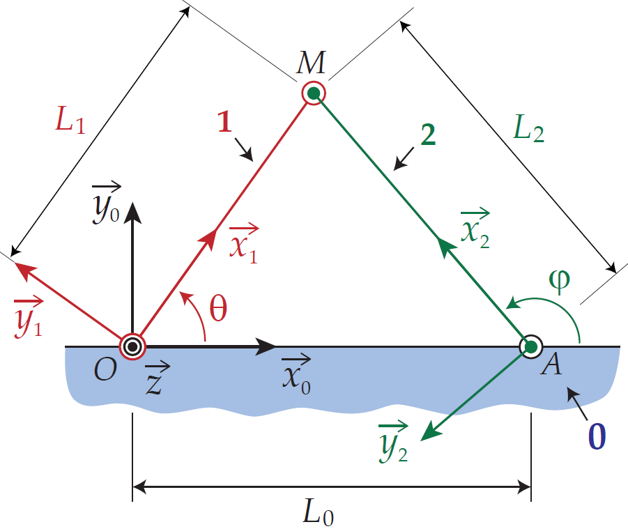 One interesting aspect of this problem is that it can be solved in Abaqus using either Truss, Beam, or Spring elements:
- With Truss elements, a single sketch is sufficient to define both beams, and the pin joints at points O, A, and M are defined implicitly.
- With Beam elements, a separate sketch must be created for each beam. The Assembly module is then used to position the beams, and a pin joint is added between them. Compared with Truss elements (and many other Abaqus element types), Beam elements have both translational and rotational degrees of freedom. This additional complexity enables them to simulate bending and torsional deformations, although these capabilities are not used in this first lab.
- Finally, Spring elements model tension-compression members as springs. Unlike Truss elements, they are not defined by a material with a Young’s modulus E and a beam cross-sectional area S, but instead by a stiffness constant K.
Lab 2: Trusses The second practical session focuses on truss structures, that is, assemblies composed of a large number of beams.
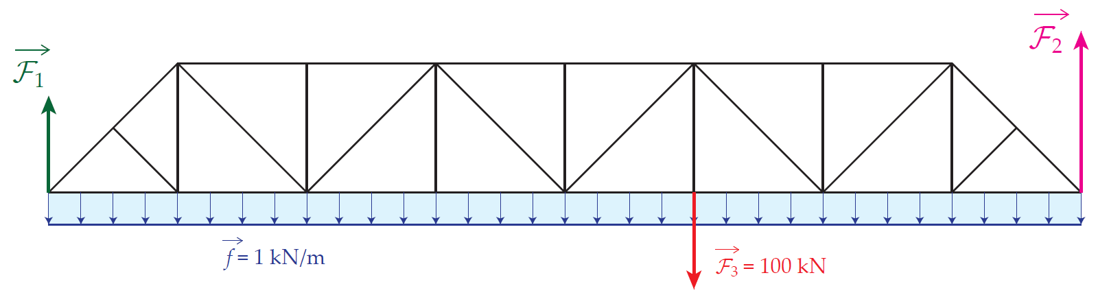
When these beams are connected by pin joints, the simplest modeling approach is to use Truss elements, since all beams can be defined within a single sketch. Sketch line duplication tools can be used to simplify the creation of sketches containing many members.
Lab 3: Bending The third practical session is devoted to the study of a cantilever beam, fixed at its left end and subjected to bending by vertical loads applied at its right end.
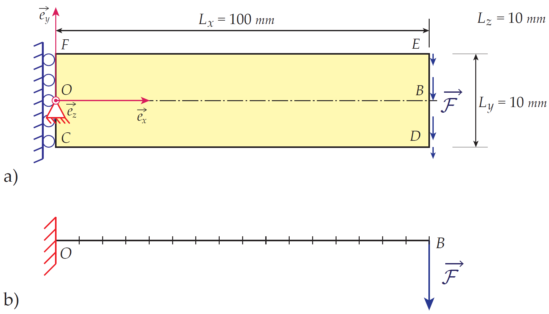
Two different modeling approaches will be used during this practical session:
- A two-dimensional model based on continuum mechanics under small-strain assumptions. It should be noted that an analytical solution to this problem is available and can be found in [Timoshenko and Goodier, 1951]. In Abaqus, the numerical model will be based on linear triangular finite elements.
- A one-dimensional model based either on Timoshenko beam theory or Bernoulli beam theory. In the 1D case, analytical solutions based on both Timoshenko and Bernoulli theories are also available. The numerical simulations in Abaqus will be carried out using Beam elements based first on Timoshenko theory and then on Bernoulli theory.
During the practical session, the three analytical deflection solutions based on the three theories (continuum mechanics, Timoshenko, and Bernoulli) will first be plotted in a spreadsheet. The three corresponding numerical solutions will then be plotted. Finally, the errors will be evaluated using the two-dimensional analytical solution as the reference.
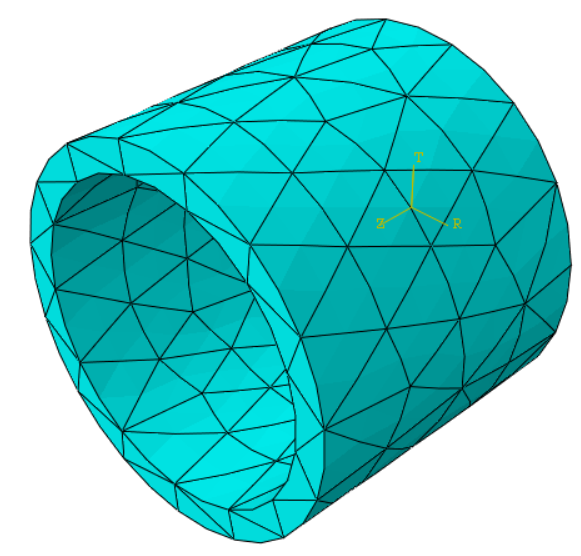
Lab 4: Torsion The fourth practical session is devoted to the study of a hollow cylinder subjected to torsion.
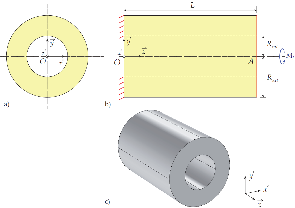
The analytical solution to this problem, based on a three-dimensional continuum mechanics analysis, will serve as the reference solution. In Abaqus, a three-dimensional numerical simulation will first be carried out, followed by a one-dimensional simulation using Beam elements.
Plates and Shells (3 sessions)
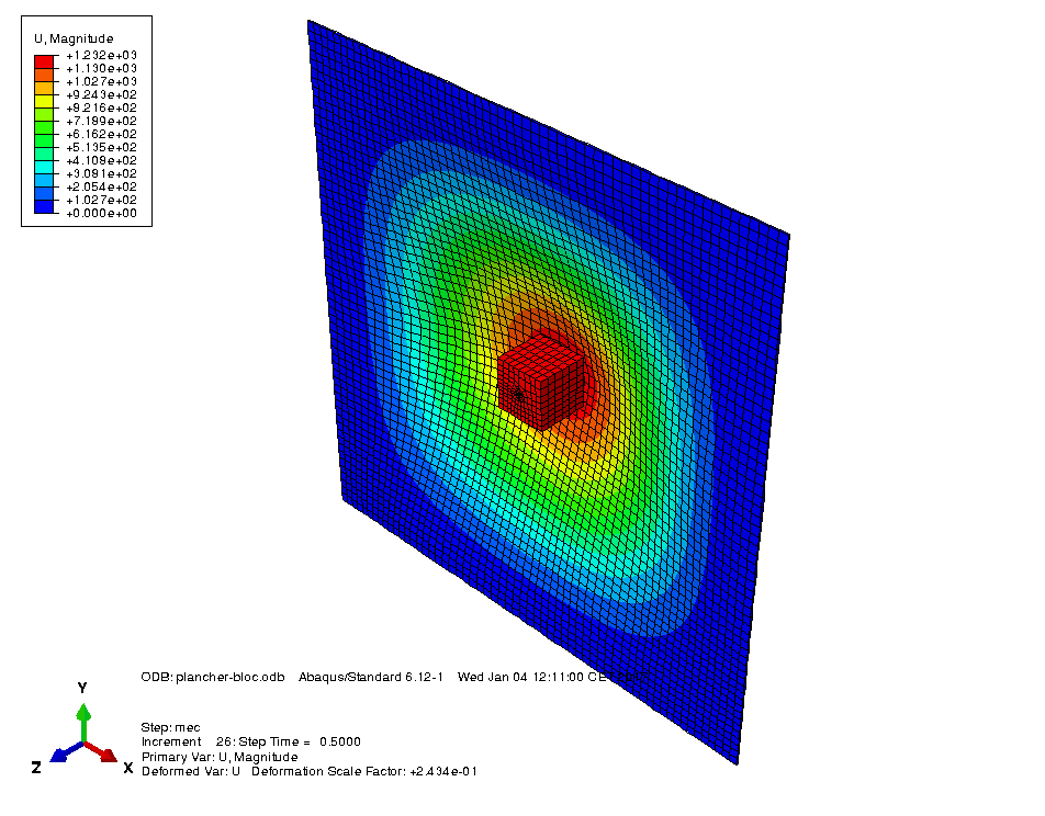
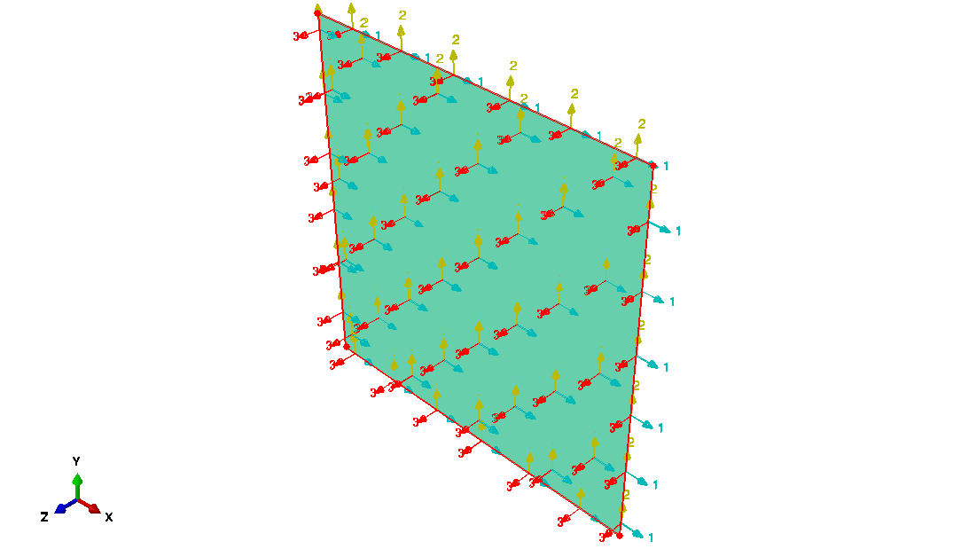
A similar approach is used for plate theory simulation, considering the elements associated to either Kirchhoff–Love or Mindlin–Reissner plate Theories.
Advanced Boundary Conditions (2 sessions)
One of the most common challenges in setting up a finite element model is the accurate definition of the boundary conditions applied to the problem. In some cases, these boundary conditions are relatively simple, consisting of prescribed displacements or applied loads over part of the domain. During the two practical sessions devoted to this topic, students will learn how to define advanced boundary conditions for problems involving more complex boundaries, including contact problems and periodic geometries.
Lab 1: Contact The first practical session focuses on a contact problem involving a trapezoidal specimen containing a notch into which a rigid punch is inserted.
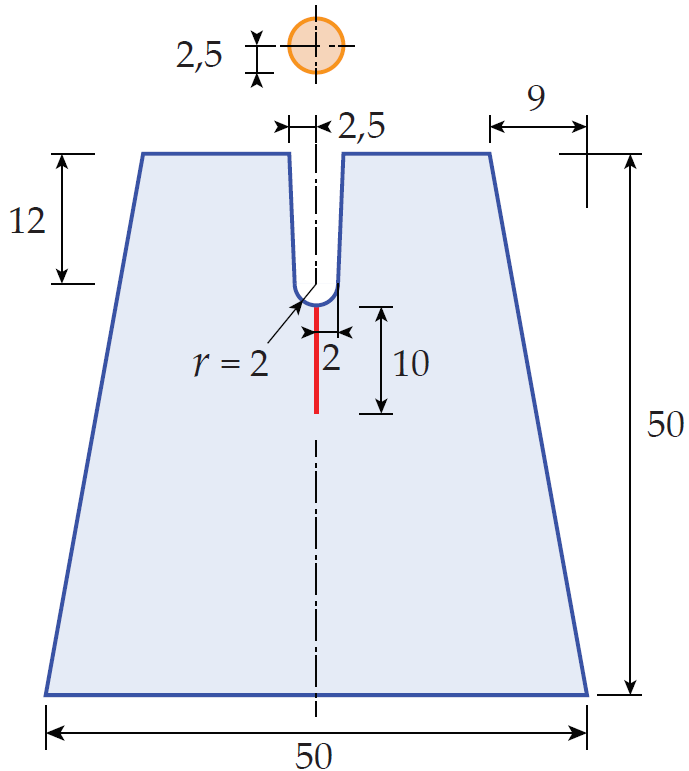
Since the sides of the notch are inclined, they tend to separate when the punch comes into contact with the specimen, eventually causing fracture once a critical deformation level is reached. In this practical session, the analysis is restricted to the pre-fracture stage, with the objective of simulating the contact between the deformable specimen and the rigid punch. This problem will later be revisited in the context of crack propagation. Students are assumed to be familiar with contact mechanics (in particular the Kuhn-Tucker conditions and Coulomb friction) as well as numerical constrained optimization methods (notably the penalty method and the Lagrange multiplier method). Several modeling approaches will be investigated in Abaqus:

- The punch will be introduced into the model as a Part of type Analytical Rigid or Discrete Rigid.
- The contact can be defined as either Node-to-Surface or Surface-to-Surface, with a friction coefficient f equal to 0 or 0.45.
The force-displacement curves obtained with each modeling approach will be superimposed and compared.
Lab 2: Periodic Structure The second practical session focuses on the study of a periodic structure, a type of structure with applications, for example, in the field of composite materials. This structure is based on a pattern (here, a square containing a circular hole at its center) that is repeated many times throughout the structure. From a numerical point of view, the mesh density depends on the size of the repeating pattern, and if the total number of patterns is large, the mesh will contain a very large number of elements, which may compromise the feasibility of the simulation.
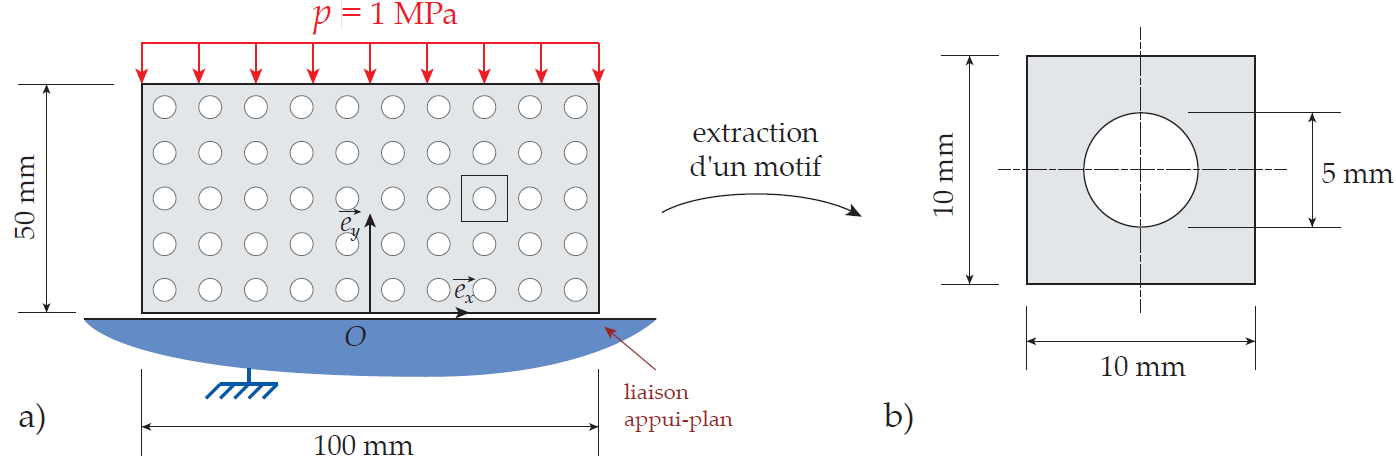
Performing a simulation on the entire structure shows that the patterns located away from the boundary of the domain all deform approximately in the same way.
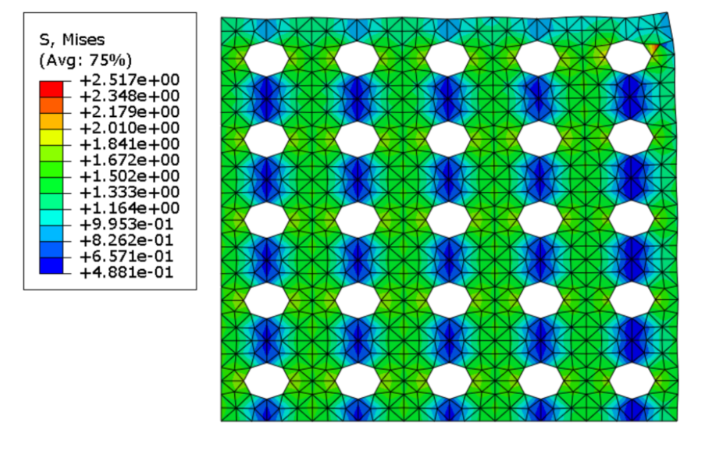
Therefore, as a first approximation, it can be assumed that not only the geometry of the problem but also its solution is periodic. In this practical session, the objective is therefore to replace the study of the complete structure by the study of a single pattern, by applying boundary conditions to the pattern that reproduce the behavior of a pattern located inside the structure.
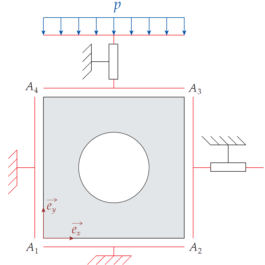
To apply these boundary conditions in Abaqus, a Reference Point will be introduced into the model. Its displacements will represent the extensions of the right and top edges. An Equation will then be added to the model to link the displacements of these two domain edges to the displacement of the Reference Point.
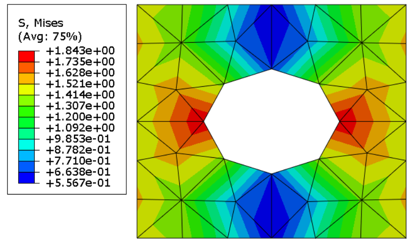
At the end of the practical session, a structure with a slightly more complex asymmetric pattern will be studied.
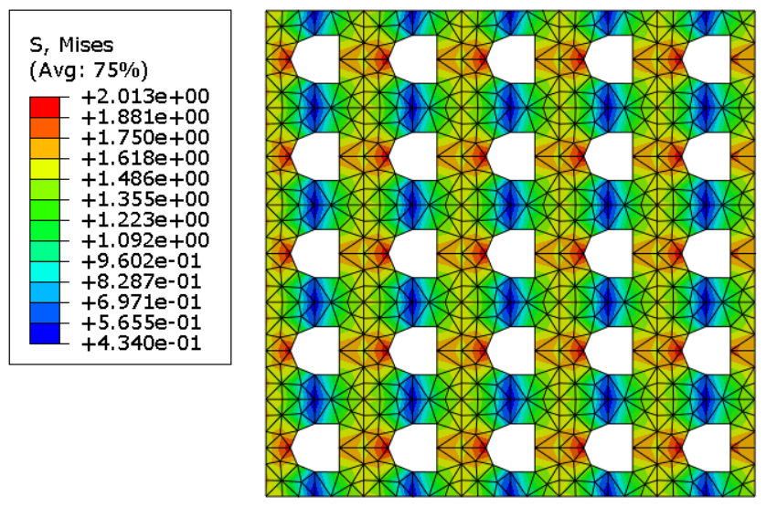
Due to the loss of symmetry, the method previously used to apply boundary conditions on the edge of a pattern will only provide approximate results for this pattern geometry. To go further in the study of deformations of periodic patterns, the “Homogenization” practical session should be considered.
Lab 3 (optional): Homogenization The final practical assignment, which does not correspond to a dedicated computer lab session, allows students to go further in defining the boundary conditions applied to a pattern of a periodic structure. For this purpose, a free Abaqus toolbox called Homtools is used, allowing the definition of three types of boundary conditions for periodic structure patterns. The most accurate of these methods corresponds to periodic boundary conditions applied to the boundaries of the domain.
Plasticity (2 sessions)
The objective of these practical sessions is to reproduce in Abaqus the behavior of a tensile specimen during a mechanical test. The starting point will be the results of a mechanical test performed on a steel specimen in a tensile testing machine. The goal of the two practical sessions is to perform numerical simulations including material nonlinearities so that the force-displacement curves obtained from the simulations overlap with the experimental reference curves.

Lab 1 During the first practical session, the 2D geometry is drawn in a sketch, the elastic part of the material behavior and the boundary conditions are defined in order to perform an initial elastic simulation. This elastic simulation provides an approximate estimate of the stress-strain law characterizing the material behavior. The obtained stress-strain law is then used as input data for an elastoplastic simulation to be defined in Abaqus.
Lab 2 During the second practical session, material damage and element deletion are added to account for fracture. This allows the modeling to be extended to large deformations, when the material behavior becomes softening (when stress becomes a decreasing function of strain).

Dynamics
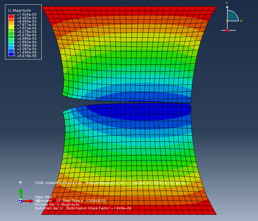
Fracture
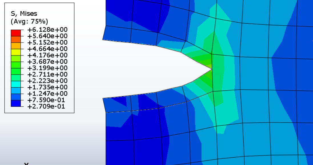
Lab 1 The first fracture mechanics practical session allows students, without considering crack propagation, to test different methods for introducing a crack into a material. The first method used is the Seam Crack method, which introduces a crack between selected elements of the mesh. This is the method used to obtain the simulation result shown below:
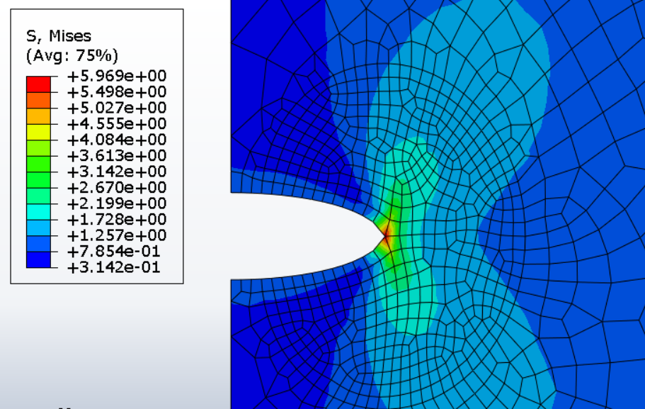
This method has the advantage that it allows the numerical calculation of the J-integral to estimate the elastic energy release rate G. This calculation is performed during the practical session, and the result is compared with the theoretical value for a simple geometry. This session also provides an opportunity to verify that the displacement field obtained from the software corresponds to the theoretical results predicted by Westergaard calculations (parabolic crack profile) and Williams calculations (asymptotic crack-tip solution).
A second alternative meshing method based on a “radial” mesh is then tested, leading to the result shown below:
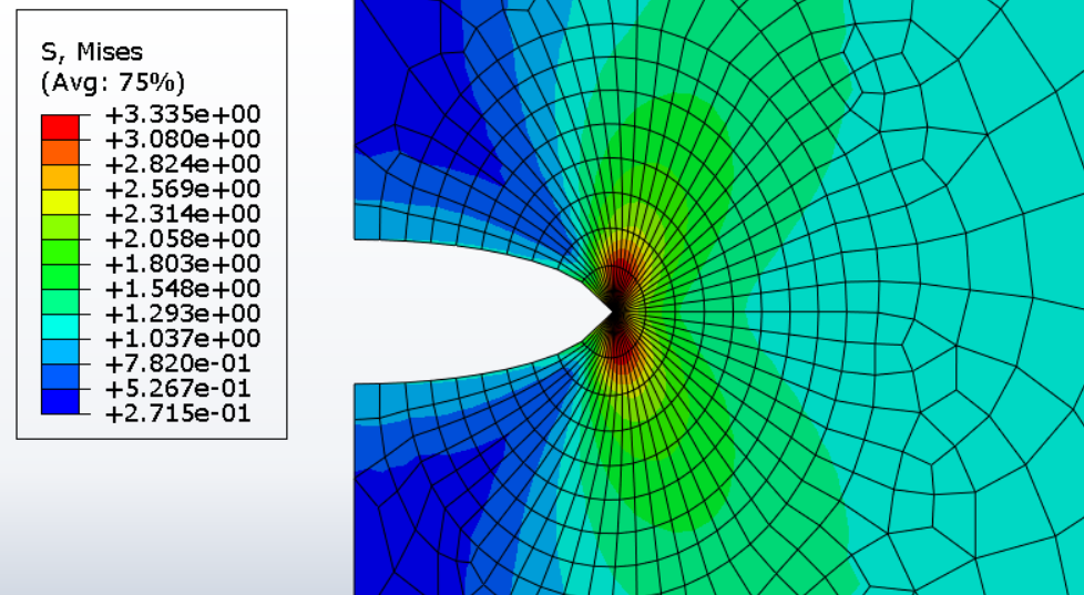
Finally, an alternative method for introducing a crack into the mesh, called the X-FEM method, is tested. This method modifies the finite elements (shape functions and numerical integration) so that the crack can pass through the finite elements of the mesh.
Lab 2 During the second practical session on fracture mechanics, the test geometry studied in Session 1 of the advanced boundary conditions practical work is reused. A pre-crack is added to the specimen to initiate fracture propagation. The purpose of this test case is to study crack propagation in the specimen, with a crack propagating vertically from top to bottom starting from the tip of the pre-crack.
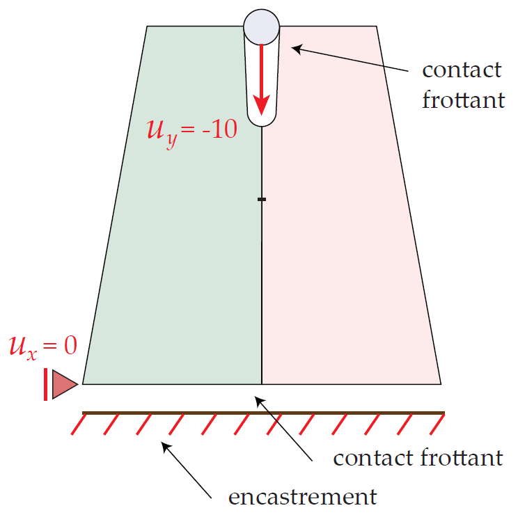 In Abaqus, a mesh is created such that the known vertical crack path passes between mesh elements. Therefore, it is only necessary to duplicate the mesh nodes while correctly applying the boundary conditions to propagate the crack. First, crack propagation is simulated using the “Virtual Crack Closure Technique”, according to the energy-based theory of fracture or Griffith theory. An alternative method based on the use of cohesive elements is then studied.

Lab 3 During the third practical session, the same problem as in the previous session is studied again, with a crack propagating vertically from top to bottom in a trapezoidal specimen. The difference compared with the previous session is that the mesh is created so that the vertical crack path along the specimen’s symmetry plane passes through a band of mesh elements. The fracture problem will therefore be defined using the extended finite element method (X-FEM).

Here again, two different crack propagation models will be used for the simulations: first, the Griffith model using the VCCT method available in Abaqus, and then a cohesive model. To define the cohesive model, it will be shown that two approaches are possible: one based on modifying the material properties and the other based on defining an interface law.